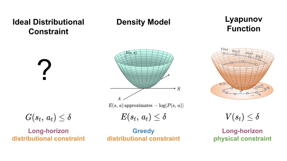
To regulate the distribution shift experience by learning-based controllers, we seek a mechanism for constraining the agent to regions of high data density throughout its trajectory (left). Here, we present an approach which achieves this goal by combining features of density models (middle) and Lyapunov functions (right).

In order to make use of machine learning and reinforcement learning in controlling real world systems, we must design algorithms which not only achieve good performance, but also interact with the system in a safe and reliable manner. Most prior work on safety-critical control focuses on maintaining the safety of the physical system, e.g. avoiding falling over for legged robots, or colliding into obstacles for autonomous vehicles. However, for learning-based controllers, there is another source of safety concern: because machine learning models are only optimized to output correct predictions on the training data, they are prone to outputting erroneous predictions when evaluated on out-of-distribution inputs. Thus, if an agent visits a state or takes an action that is very different from those in the training data, a learning-enabled controller may “exploit” the inaccuracies in its learned component and output actions that are suboptimal or even dangerous.

To prevent these potential “exploitations” of model inaccuracies, we propose a new framework to reason about the safety of a learning-based controller with respect to its training distribution. The central idea behind our work is to view the training data distribution as a safety constraint, and to draw on tools from control theory to control the distributional shift experienced by the agent during closed-loop control. More specifically, we’ll discuss how Lyapunov stability can be unified with density estimation to produce Lyapunov density models, a new kind of safety “barrier” function which can be used to synthesize controllers with guarantees of keeping the agent in regions of high data density. Before we introduce our new framework, we will first give an overview of existing techniques for guaranteeing physical safety via barrier function.

Guaranteeing Safety via Barrier Functions

In control theory, a central topic of study is: given known system dynamics, $s_{t+1}=f(s_t, a_t)$, and known system constraints, $s \in C$, how can we design a controller that is guaranteed to keep the system within the specified constraints? Here, $C$ denotes the set of states that are deemed safe for the agent to visit. This problem is challenging because the specified constraints need to be satisfied over the agent’s entire trajectory horizon ($s_t \in C$ $\forall 0\leq t \leq T$). If the controller uses a simple “greedy” strategy of avoiding constraint violations in the next time step (not taking $a_t$ for which $f(s_t, a_t) \notin C$), the system may still end up in an “irrecoverable” state, which itself is considered safe, but will inevitably lead to an unsafe state in the future regardless of the agent’s future actions. In order to avoid visiting these “irrecoverable” states, the controller must employ a more “long-horizon” strategy which involves predicting the agent’s entire future trajectory to avoid safety violations at any point in the future (avoid $a_t$ for which all possible $\{ a_{\hat{t}} \}_{\hat{t}=t+1}^H$ lead to some $\bar{t}$ where $s_{\bar{t}} \notin C$ and $t<\bar{t} \leq T$). However, predicting the agent’s full trajectory at every step is extremely computationally intensive, and often infeasible to perform online during run-time.

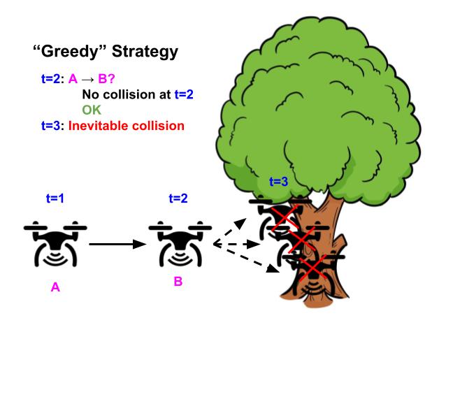
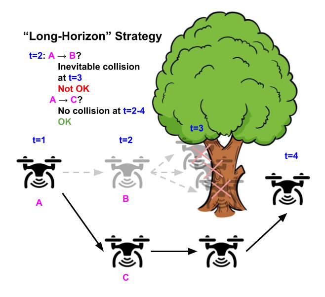
Illustrative example of a drone whose goal is to fly as straight as possible while avoiding obstacles. Using the “greedy” strategy of avoiding safety violations (left), the drone flies straight because there’s no obstacle in the next timestep, but inevitably crashes in the future because it can’t turn in time. In contrast, using the “long-horizon” strategy (right), the drone turns early and successfully avoids the tree, by considering the entire future horizon future of its trajectory.

Control theorists tackle this challenge by designing “barrier” functions, $v(s)$, to constrain the controller at each step (only allow $a_t$ which satisfy $v(f(s_t, a_t)) \leq 0$). In order to ensure the agent remains safe throughout its entire trajectory, the constraint induced by barrier functions ($v(f(s_t, a_t))\leq 0$) prevents the agent from visiting both unsafe states and irrecoverable states which inevitably lead to unsafe states in the future. This strategy essentially amortizes the computation of looking into the future for inevitable failures when designing the safety barrier function, which only needs to be done once and can be computed offline. This way, at runtime, the policy only needs to employ the greedy constraint satisfaction strategy on the barrier function $v(s)$ in order to ensure safety for all future timesteps.

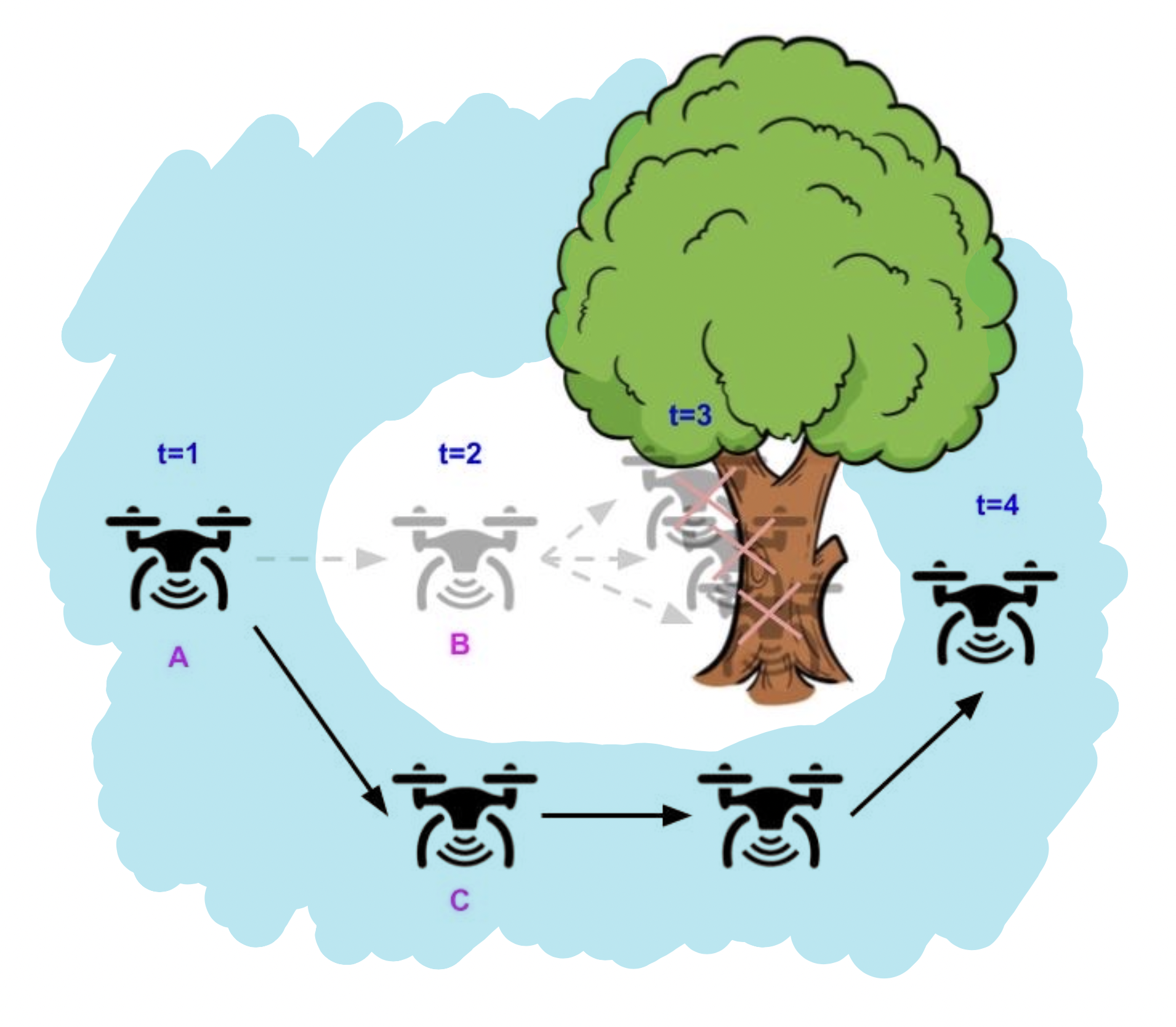
The blue region denotes the of states allowed by the barrier function constraint, $\{s | v(s) \leq 0\}$. Using a “long-horizon” barrier function, the drone only needs to greedily ensure that the barrier function constraint $v(s) \leq 0$ is satisfied for the next state, in order to avoid safety violations for all future timesteps.

Here, we used the notion of a “barrier” function as an umbrella term to describe a number of different kinds of functions whose functionalities are to constrain the controller in order to make long-horizon guarantees. Some specific examples include control Lyapunov functions for guaranteeing stability, control barrier functions for guaranteeing general safety constraints, and the value function in Hamilton-Jacobi reachability for guaranteeing general safety constraints under external disturbances. More recently, there has also been some work on learning barrier functions, for settings where the system is unknown or where barrier functions are difficult to design. However, prior works in both traditional and learning-based barrier functions are mainly focused on making guarantees of physical safety. In the next section, we will discuss how we can extend these ideas to regulate the distribution shift experienced by the agent when using a learning-based controller.

Lyapunov Density Models

To prevent model exploitation due to distribution shift, many learning-based control algorithms constrain or regularize the controller to prevent the agent from taking low-likelihood actions or visiting low likelihood states, for instance in offline RL, model-based RL, and imitation learning. However, most of these methods only constrain the controller with a single-step estimate of the data distribution, akin to the “greedy” strategy of keeping an autonomous drone safe by preventing actions which causes it to crash in the next timestep. As we saw in the illustrative figures above, this strategy is not enough to guarantee that the drone will not crash (or go out-of-distribution) in another future timestep.

How can we design a controller for which the agent is guaranteed to stay in-distribution for its entire trajectory? Recall that barrier functions can be used to guarantee constraint satisfaction for all future timesteps, which is exactly the kind of guarantee we hope to make with regards to the data distribution. Based on this observation, we propose a new kind of barrier function: the Lyapunov density model (LDM), which merges the dynamics-aware aspect of a Lyapunov function with the data-aware aspect of a density model (it is in fact a generalization of both types of function). Analogous to how Lyapunov functions keeps the system from becoming physically unsafe, our Lyapunov density model keeps the system from going out-of-distribution.

An LDM ($G(s, a)$) maps state and action pairs to negative log densities, where the values of $G(s, a)$ represent the best data density the agent is able to stay above throughout its trajectory. It can be intuitively thought of as a “dynamics-aware, long-horizon” transformation on a single-step density model ($E(s, a)$), where $E(s, a)$ approximates the negative log likelihood of the data distribution. Since a single-step density model constraint ($E(s, a) \leq -\log(c)$ where $c$ is a cutoff density) might still allow the agent to visit “irrecoverable” states which inevitably causes the agent to go out-of-distribution, the LDM transformation increases the value of those “irrecoverable” states until they become “recoverable” with respect to their updated value. As a result, the LDM constraint ($G(s, a) \leq -\log(c)$) restricts the agent to a smaller set of states and actions which excludes the “irrecoverable” states, thereby ensuring the agent is able to remain in high data-density regions throughout its entire trajectory.

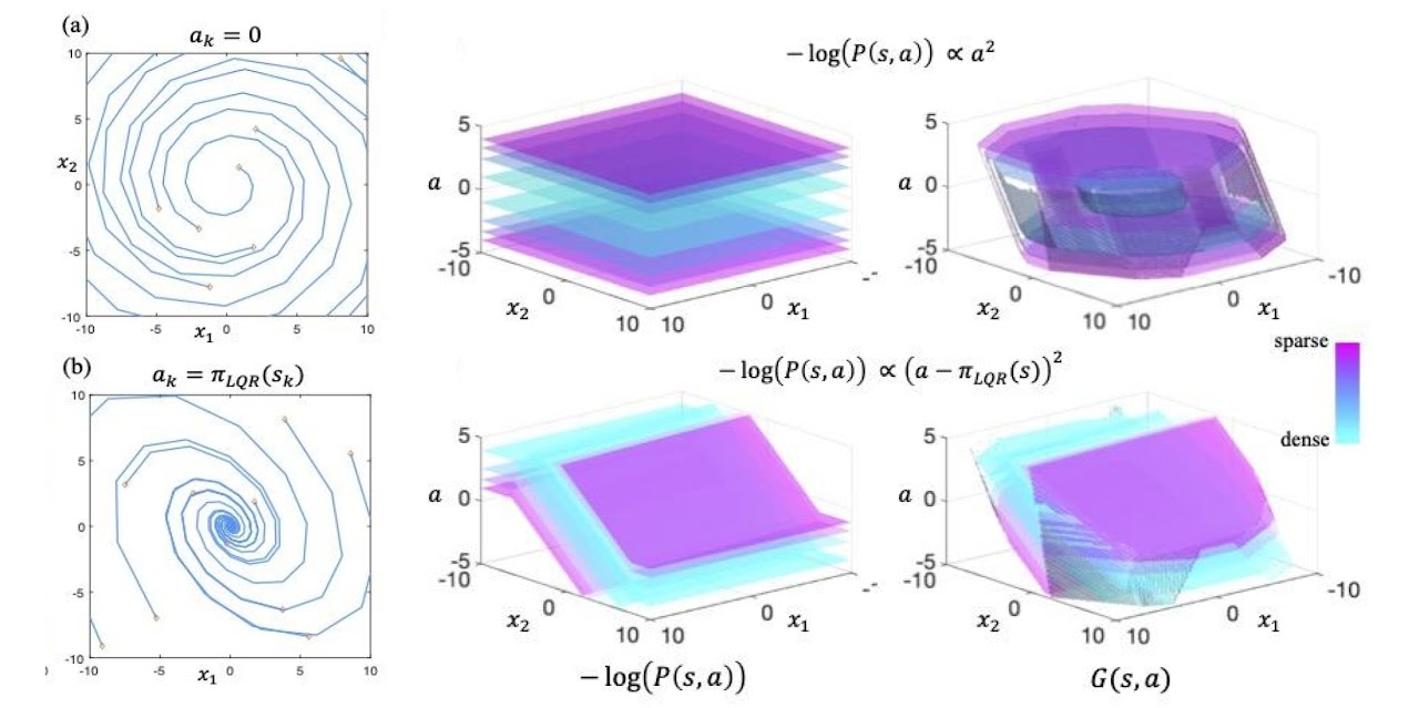
Example of data distributions (middle) and their associated LDMs (right) for a 2D linear system (left). LDMs can be viewed as "dynamics-aware, long-horizon" transformations on density models.

How exactly does this “dynamics-aware, long-horizon” transformation work? Given a data distribution $P(s, a)$ and dynamical system $s_{t+1} = f(s_t, a_t)$, we define the following as the LDM operator: $\mathcal{T}G(s, a) = \max\{-\log P(s, a), \min_{a’} G(f(s, a), a’)\}$. Suppose we initialize $G(s, a)$ to be $-\log P(s, a)$. Under one iteration of the LDM operator, the value of a state action pair, $G(s, a)$, can either remain at $-\log P(s, a)$ or increase in value, depending on whether the value at the best state action pair in the next timestep, $\min_{a’} G(f(s, a), a’)$, is larger than $-\log P(s, a)$. Intuitively, if the value at the best next state action pair is larger than the current $G(s, a)$ value, this means that the agent is unable to remain at the current density level regardless of its future actions, making the current state “irrecoverable” with respect to the current density level. By increasing the current the value of $G(s, a)$, we are “correcting” the LDM such that its constraints would not include “irrecoverable” states. Here, one LDM operator update captures the effect of looking into the future for one timestep. If we repeatedly apply the LDM operator on $G(s, a)$ until convergence, the final LDM will be free of “irrecoverable” states in the agent’s entire future trajectory.

To use an LDM in control, we can train an LDM and learning-based controller on the same training dataset and constrain the controller’s action outputs with an LDM constraint ($G(s, a)) \leq -\log(c)$). Because the LDM constraint prevents both states with low density and “irrecoverable” states, the learning-based controller will be able to avoid out-of-distribution inputs throughout the agent’s entire trajectory. Furthermore, by choosing the cutoff density of the LDM constraint, $c$, the user is able to control the tradeoff between protecting against model error vs. flexibility for performing the desired task.

Example evaluation of ours and baseline methods on a hopper control task for different values of constraint thresholds (x- axis). On the right, we show example trajectories from when the threshold is too low (hopper falling over due to excessive model exploitation), just right (hopper successfully hopping towards target location), or too high (hopper standing still due to over conservatism).

So far, we have only discussed the properties of a “perfect” LDM, which can be found if we had oracle access to the data distribution and dynamical system. In practice, though, we approximate the LDM using only data samples from the system. This causes a problem to arise: even though the role of the LDM is to prevent distribution shift, the LDM itself can also suffer from the negative effects of distribution shift, which degrades its effectiveness for preventing distribution shift. To understand the degree to which the degradation happens, we analyze this problem from both a theoretical and empirical perspective. Theoretically, we show even if there are errors in the LDM learning procedure, an LDM constrained controller is still able to maintain guarantees of keeping the agent in-distribution. Albeit, this guarantee is a bit weaker than the original guarantee provided by a perfect LDM, where the amount of degradation depends on the scale of the errors in the learning procedure. Empirically, we approximate the LDM using deep neural networks, and show that using a learned LDM to constrain the learning-based controller still provides performance improvements compared to using single-step density models on several domains.

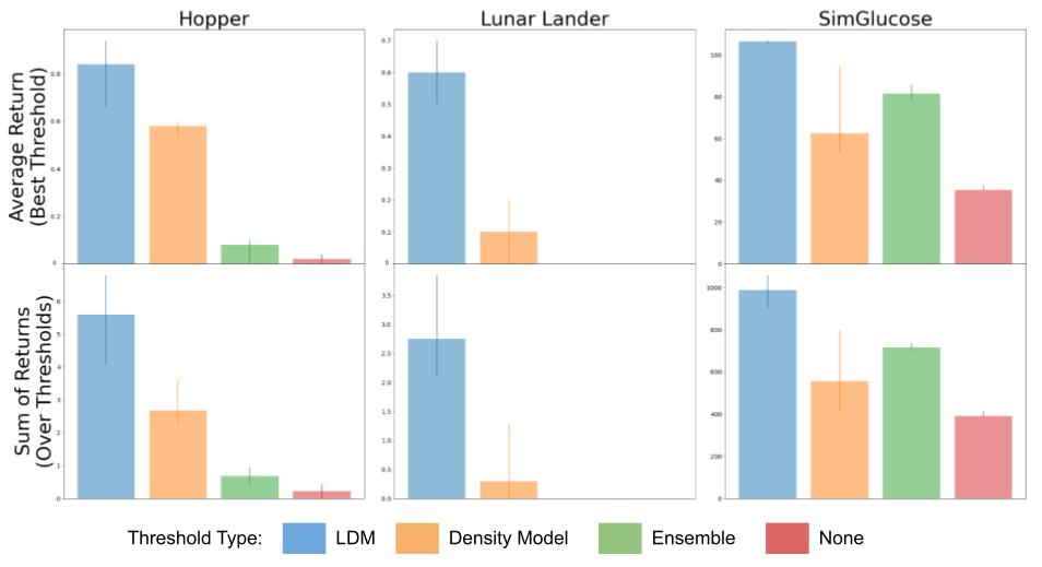
Evaluation of our method (LDM) compared to constraining a learning-based controller with a density model, the variance over an ensemble of models, and no constraint at all on several domains including hopper, lunar lander, and glucose control.

Conclusion and Takeaways

Currently, one of the biggest challenges in deploying learning-based controllers on real world systems is their potential brittleness to out-of-distribution inputs, and lack of guarantees on performance. Conveniently, there exists a large body of work in control theory focused on making guarantees about how systems evolve. However, these works usually focus on making guarantees with respect to physical safety requirements, and assume access to an accurate dynamics model of the system as well as physical safety constraints. The central idea behind our work is to instead view the training data distribution as a safety constraint. This allows us to make use of these ideas in controls in our design of learning-based control algorithms, thereby inheriting both the scalability of machine learning and the rigorous guarantees of control theory.

This post is based on the paper “Lyapunov Density Models: Constraining Distribution Shift in Learning-Based Control”, presented at ICML 2022. You find more details in our paper and on our website. We thank Sergey Levine, Claire Tomlin, Dibya Ghosh, Jason Choi, Colin Li, and Homer Walke for their valuable feedback on this blog post.