We introduce Bit-Swap, a scalable and effective lossless data compression technique based on deep learning. It extends previous work on practical compression with latent variable models, based on bits-back coding and asymmetric numeral systems. In our experiments Bit-Swap is able to beat benchmark compressors on a highly diverse collection of images. We’re releasing code for the method and optimized models such that people can explore and advance this line of modern compression ideas. We also release a demo and a pre-trained model for Bit-Swap image compression and decompression on your own image. See the end of the post for a talk that covers how bits-back coding and Bit-Swap works.
Lossless compression for high-dimensional data
The goal is to design an effective lossless compression scheme that is scalable to high-dimensional data, like images. This is a matter of concurrently solving two problems:
-
choosing a statistical model that closely captures the underlying distribution of the input data and
-
developing a scalable compression algorithm that exploits this model’s theoretical compression potential.
The compression ratio of the resulting compression scheme heavily relies on the first problem: the model capacity. Recent advances in deep learning allow us to optimize probabilistic models of complex high-dimensional data efficiently. These developments have opened up many opportunities regarding lossless compression. A powerful technique is to pair autoregressive models with entropy coders, like arithmetic coding or asymmetric numeral systems (ANS), resulting in excellent compression ratios. However, the autoregressive structure typically makes decompression several orders of magnitude slower than compression.
Fortunately, ANS is known to be amenable to parallelization. To exploit this property, we have to narrow our focus to models that encompass fully factorized distributions. This constraint forces us to be extra innovative and choose our model and coding scheme accordingly.
Recent work
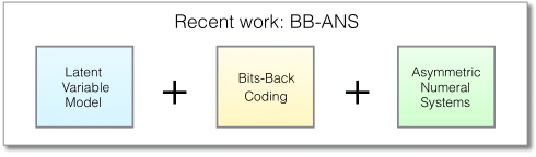
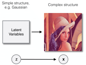
The recent Bits-Back with Asymmetric Numeral Systems (BB-ANS) method tries to mitigate this issue by combining latent variable models with ANS. Latent variable models define unobserved random variables whose values help govern the distribution of the data. For example, if the observed data consists of images, the composition of the images may be dependent on the locations of edges and textures, which are latent variables. (In practice, we typically define an uninformative prior over the latent variables, like a standard gaussian.) This type of model may use fully factorized distributions and can be efficiently optimized using the VAE framework.
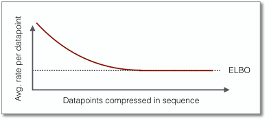
The critical component that enables BB-ANS to compress with latent variable models is a principle called bits-back coding that turned out to be a natural fit with ANS. Bits-back coding ensures compression that closely matches the negative ELBO on average, in addition to an overhead that only occurs at initialization. This overhead becomes insignificant when compressing long sequences of datapoints at once.
Our contribution
While latent variable models can be designed to be complex density estimators, restricting the model to fully factorized distributions, however, can significantly limit model flexibility. Therefore, we propose employing hierarchical latent variable models, which typically have greater modelling capacity than models with a single latent layer. We extend the latent variable model recursively, by substituting its fully factorized prior distribution by a second latent variable model, substituting its prior by a third latent variable model, and so on.
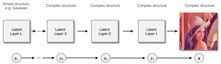
For example, if the observed data are images, the composition of the images may be dependent on the locations of edges and textures, which may be dependent on the locations of objects, which may be dependent on the scene composition, etc. Note that if we let every layer be solely dependent on the layer on top of that, this model design can be interpreted as multiple nested latent variable models: the observed data distribution being governed by latent layer 1, latent layer 1 distribution being governed by latent layer 2, up until the top latent layer, which has an unconditional prior distribution.
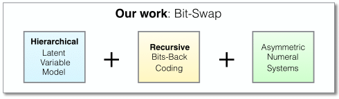
Using that insight, we developed a novel coding technique called recursive bits-back coding. As the name suggests, we apply bits-back coding on every layer recursively, processing the nested latent variable models from bottom to top. We coined the joint composition of recursive bits-back coding and the specified hierarchical latent variable model Bit-Swap. The merits of Bit-Swap include:
-
Applying bits-back coding in a recursive manner resulting in an overhead that is bounded and in practice does not grow with the depth of the model hierarchy. This stands in contrast with naively applying BB-ANS on a hierarchical latent variable model, which would ignore the latent variable topology and would treat all latent layers as one single vector, resulting in an overhead that linearly grows with the depth of the hierarchy. The bounded overhead makes Bit-Swap particularly interesting if we want to employ a powerful model with a deep latent hierarchy, while we do not wish to compress long sequences of datapoints at once.
-
Bit-Swap is still able to compress close to the negative ELBO on average, in addition to a smaller overhead.
-
Nesting the latent variable models through the prior distribution of every layer enables more complex distributions for every latent layer, except for the top one. The nested structure prompts a tighter ELBO, which in turn results in lower compression ratios.
-
We maintain fully factorized distributions throughout the model, which makes the entire coding process is parallelizable. Using a GPU implementation of ANS, together with model-parallelism, should result in high-speed compression and decompression. The major bottleneck in our implementation is the ANS operation, but we are optimistic this can be resolved due to its inherent parallelizability. We leave speed optimization of Bit-Swap to future work.
Results
| Compression ratio of 100 images from ImageNet (unscaled & cropped) | |
|---|---|
| Uncompressed | 100.00 % |
| GNU Gzip | 74.50 % |
| bzip2 | 63.38 % |
| LZMA | 63.63 % |
| PNG | 58.88 % |
| WebP | 45.75 % |
| BB-ANS | 45.25 % |
| Bit-Swap | 43.88 % |
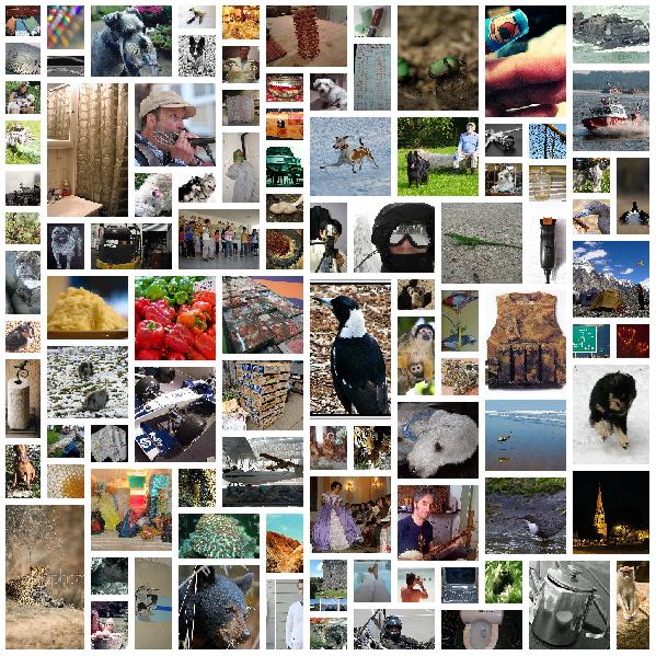
We trained the hierarchical latent variable model on random 32 by 32 pixel patches of the training set of ImageNet. For testing, we took 100 images independently from the test set. The 100 images were cropped to multiples of 32 pixels on each side, such that we could fit a grid 32 by 32 pixel blocks. The grid is treated as a dataset that has to be processed in sequence in order to be compressed with Bit-Swap and BB-ANS. We then apply Bit-Swap and BB-ANS to a single sequence at the time, corresponding to compressing one image at the time. We used the same cropped images for the baseline schemes, without first breaking the images up in 32 x 32 pixel blocks. The results are shown above. We believe results can be further improved by using bigger pixel patches and more sophisticated model optimization. All other results can be found in the paper.
Demo
Compress your own image using Bit-Swap. Clone the GitHub repository on
https://github.com/fhkingma/bitswap and
run the script demo_compress.py and demo_decompress.py. The script
demo_compress.py will compress using Bit-Swap and compare it against GNU
Gzip, bzip2, LZMA, PNG and WebP compression. The script demo_decompress.py
will decompress a Bit-Swap compressed file.
Note: if the input file is already compressed (JPEG, PNG etc.), the script first has to decompress that file export it to RGB pixel data. Thereafter, the RGB pixel values are the input and that data gets compressed by Bit-Swap and the other schemes, resulting in size reduction compared to the RGB pixel data. One might notice that the raw RGB pixel data contains (much) more information than the input file. The discrepancy between the file sizes is especially prominent when converting JPEG files to RGB data. This is largely because JPEG, a lossy compressor, consists of a quantization step, in which the original image loses a (large) portion of the information. Quantization creates predictable patterns, which are in turn compressed using lossless compression techniques for the purpose of storage. When decompressing the JPEG file and converting to RGB, however, we store every single pixel value explicitly, thus disregarding the patterns. This could result in a large increase of information.
Video
See the video below for a talk about this paper.
You can find the slides here.
This work was done while the author was at UC Berkeley. We refer the reader to the following paper for details:
- Bit-Swap: Recursive Bits-Back Coding for Lossless Compression with Hierarchical Latent Variables
Friso H. Kingma, Pieter Abbeel, Jonathan Ho
ICML 2019