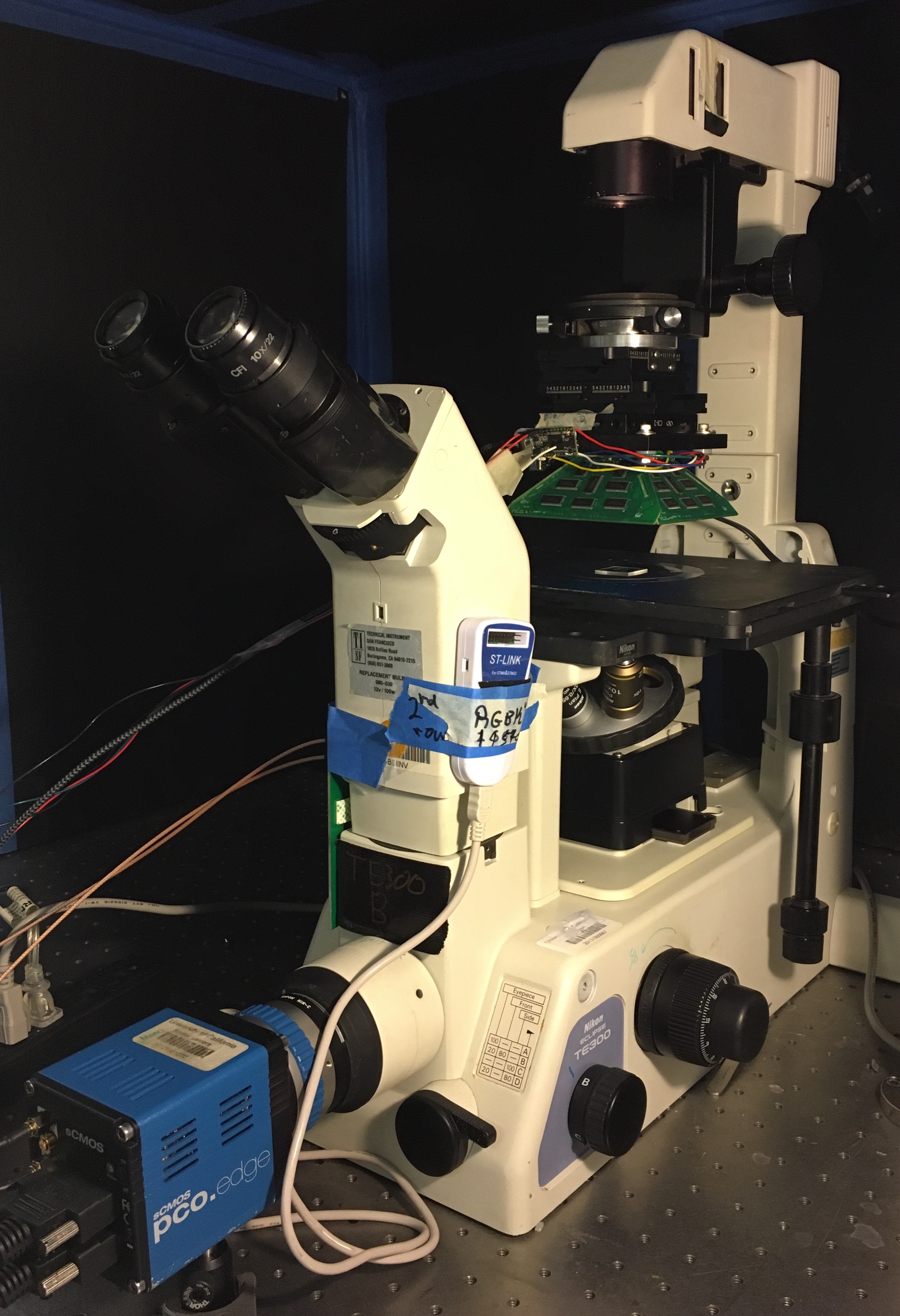
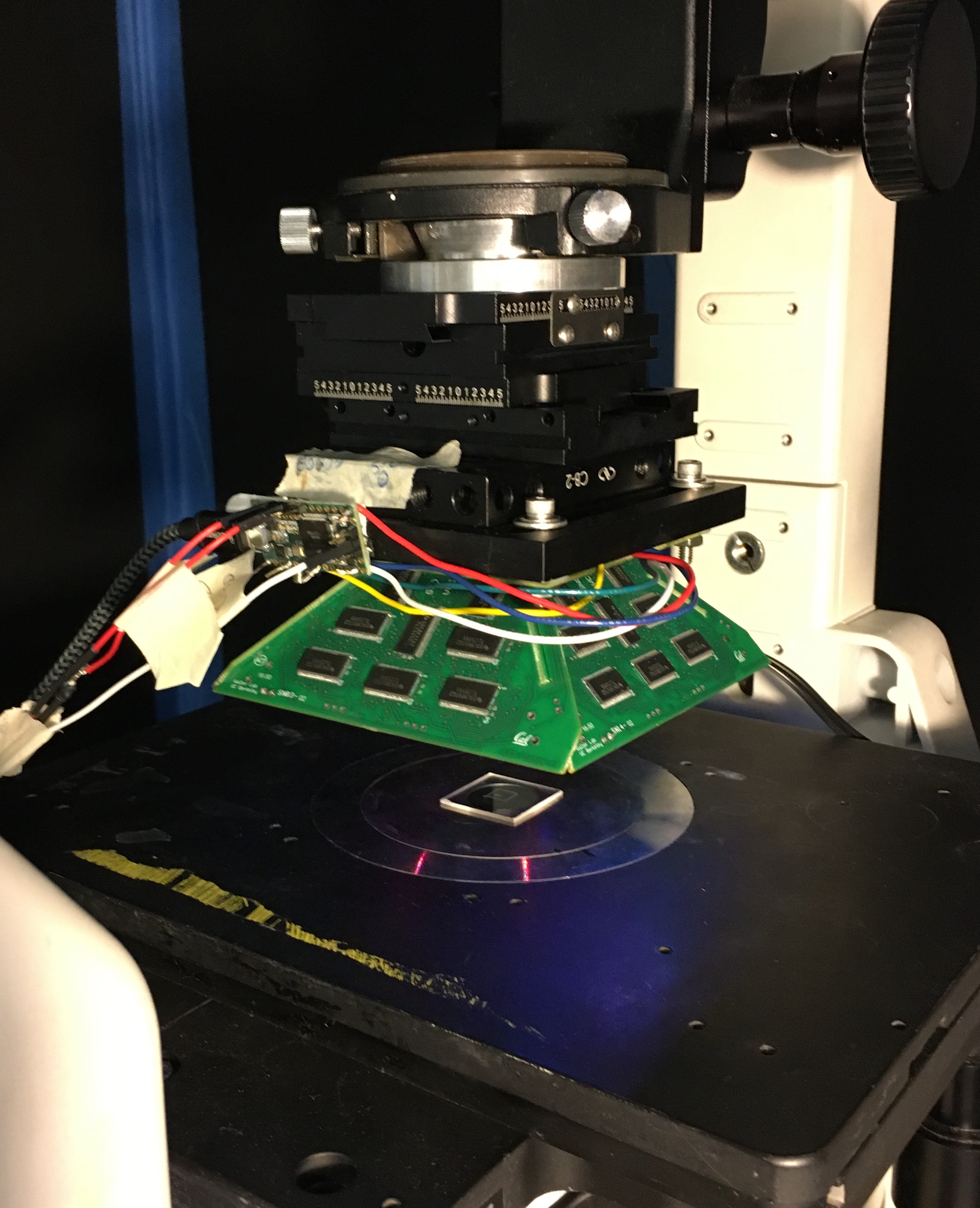
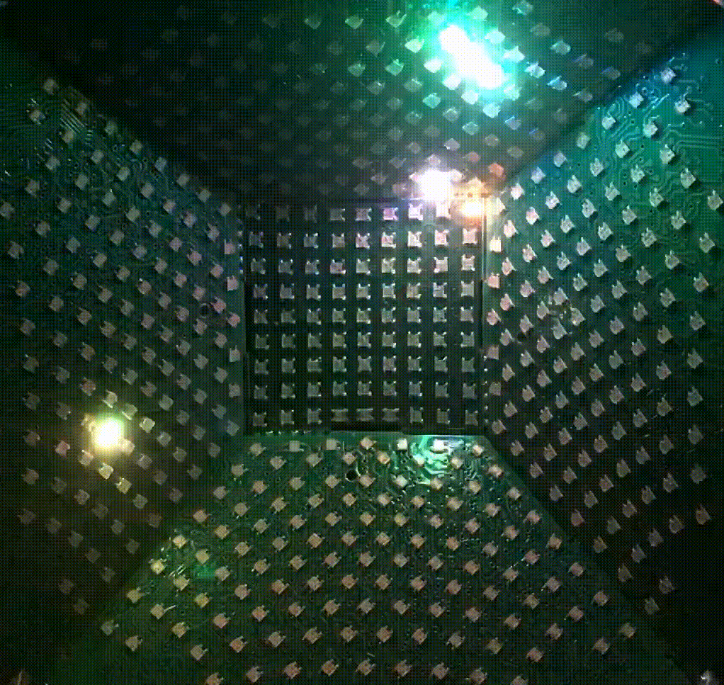
Figure 1: (left) LED Array Microscope constructed using a standard
commercial microscope and an LED array. (middle) Close up on the LED array dome
mounted on the microscope. (right) LED array displaying patterns at 100Hz.
Computational imaging systems marry the design of hardware and image reconstruction. For example, in optical microscopy, tomographic, super-resolution, and phase imaging systems can be constructed from simple hardware modifications to a commercial microscope (Fig. 1) and computational reconstruction. Traditionally, we require a large number of measurements to recover the above quantities; however, for live cell imaging applications, we are limited in the number of measurements we can acquire due to motion. Naturally, we want to know what are the best measurements to acquire. In this post, we highlight our latest work that learns the experimental design to maximize the performance of a non-linear computational imaging system.
Motivation
Standard microscopes usually image the absorption contrast of the sample; however, most biological cells are weakly absorbing. Stains or dyes can be used to observe contrast, but this may be prohibitively invasive for live cell biology. With a computational imaging system it is possible to image other intrinsic optical properties of the sample such as phase (i.e. refractive index) to provide us with a strong mechanism for contrast (Fig. 2) and quantitative information about the sample.
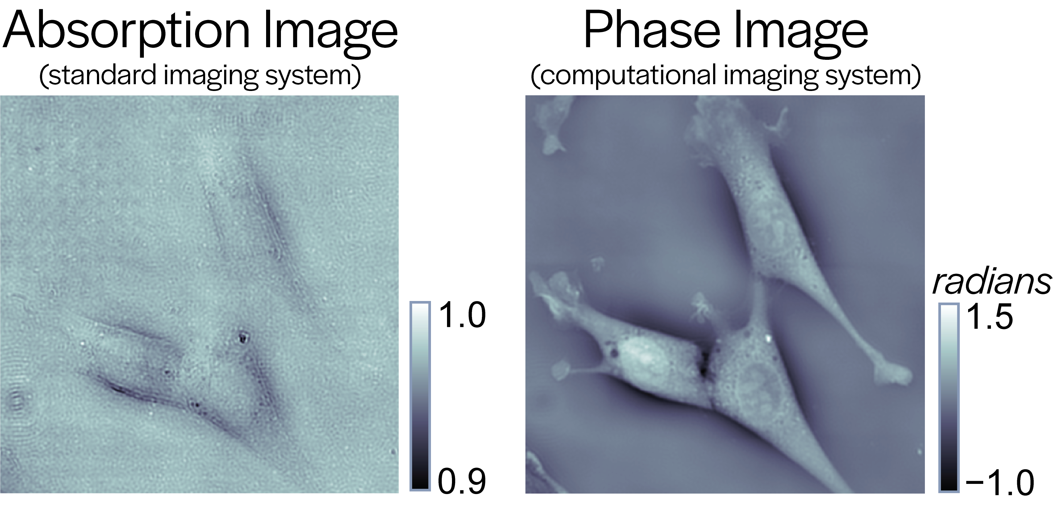
Figure 2: Mouse Fibroblast Cells: (left) absorption contrast image has poor
contrast, (right) quantitative phase image has strong structural contrast.
Using a standard microscope, the illumination source can be replaced with a programmable LED array to construct an LED array microscope (Fig 1.). Images taken under different LED’s illumination will encode information about the sample’s phase (specifically, different parts of the sample’s spatial spectrum) into the intensity measurements. A large set of measurements (10s to 100s) can then be combined by solving an inverse problem to quantitatively reconstruct the phase of the sample, possibly with higher resolution than the native resolution of the microscope, or in 3D.
Due to the multiple measurement requirement, obtaining high quality reconstructions is traded off with poor temporal resolution. So when sample motion is present, poor temporal resolution will degrade image quality due to motion blur. To improve upon this tradeoff, designing how to capture a smaller set of measurements would enable high quality reconstruction at an improved temporal resolution. But what are the best patterns to display on the LED array? What is the most efficient way to encode information?
Figure 3: LED Array Microscope System: (top) Measurement formation
process using a LED array microscope. (bottom) Regularized inverse problem
solved for image reconstruction.
Designing the LED array patterns for a set of measurements is complicated. Many computational imaging systems, including this one, are non-linear in how the hardware encodes information, how the computation reconstructs information, or both. Conventional design methods, (e.g. optimal design, spectral analysis) almost all consider design for linear system models and linear reconstructions, thus will not necessarily improve performance for systems when the processes are non-linear.
In this post, we consider a new computational imaging framework, Physics-based Learned Design [1], that learns the experimental design to maximize the overall performance of the microscope given a system model, a computational reconstruction, and a dataset. Here, we consider using the LED array microscope as our hardware system and regularized phase retrieval as our computational reconstruction (Fig. 3). Both of these systems are non-linear and thus are difficult to design using conventional methods. To demonstrate our method, we learn an experimental design for Quantitative Phase Imaging using a small simulated dataset and in experiment show similar reconstruction quality to a more sophisticated method using only a fraction of the measurements.
Optimal Experiment Design and Phase Retrieval
Optimal experiment design methods consider minimizing the variance (mean square error) of an unbiased estimator or equivalently maximizing its information (the reciprocal of the variance). Usually, methods optimize real-valued summary statistic (e.g. trace, determinant) of the variance, especially when estimating several parameters. However, such design methods are only optimal for linear unbiased estimators (e.g. least squares) and will not necessarily be optimal for non-linear biased estimators. In our setting, we want to estimate the phase image by solving a regularized phase retrieval problem (both a non-linear and biased estimator).
We want to retrieve the sample’s optical properties, $\mathbf{x}$, from several non-linear measurements, $\mathbf{y}_k$, by minimizing a data consistency term, $\mathcal{D}$, and a prior term, $\mathcal{P}$, (e.g. sparsity, total-variation).
This type of cost function can be iteratively minimized via gradient-based optimization (e.g. accelerated proximal gradient descent or alternating direction method of multipliers). Here we choose accelerated proximal gradient descent.
Algorithm 1: Accelerated Proximal Gradient Descent, $\mathbf{x}$ is the
current estimate, $\mu$ is the acceleration term, $\mathbf{w},\mathbf{z}$ are
intermediate variables, and $N$ is the number of iterations. Each iteration
consists of a gradient update (green), proximal update (pink), and an
acceleration update (orange).
Physics-based Network
Our goal is to learn the experimental design (i.e. how to best encode information) for the non-linear computational imaging system outlined in figure 3. However, as we discussed conventional design methods will not work, so let us rethink the problem. Consider unrolling the iterations of the optimizer in Alg. 1 into a network where each layer of the network is an iteration of the optimizer. Within each layer we have operations which perform a gradient update, a proximal update, and an acceleration update. Now, we have a network that incorporates the non-linear image formation process and the prior information from the reconstruction.
Figure 4: Unrolled Physics-based Network: (left) takes several camera
measurements parameterized by the hardware design, $C$, as input and (right)
outputs the reconstructed phase image, $\mathbf{x}^{(N)}$, which is compared to the
ground truth, $\mathbf{x}'$. Each layer of the network corresponds to an
iteration of the gradient-based image reconstruction. Within each layer, there is a
gradient update (green), a proximal update (pink), and an acceleration update (orange).
We are not the first to consider unrolled physics-based networks. A work in another imaging field considers unrolling the iterations of their image reconstruction to form a network and then learns quantities in the reconstruction that replace the proximal update [2]. In the past year, the mechanics of unrolling the iterations of an image reconstruction pipeline have rapidly grown in popularity.
Physics-based Learned Design
For our context, we want to learn how to turn on the LEDs during each measurement. Specifically, we learn the brightness of each LED, such that the image reconstruction error is minimized. Now, the experimental design can be posed as a supervised learning problem,
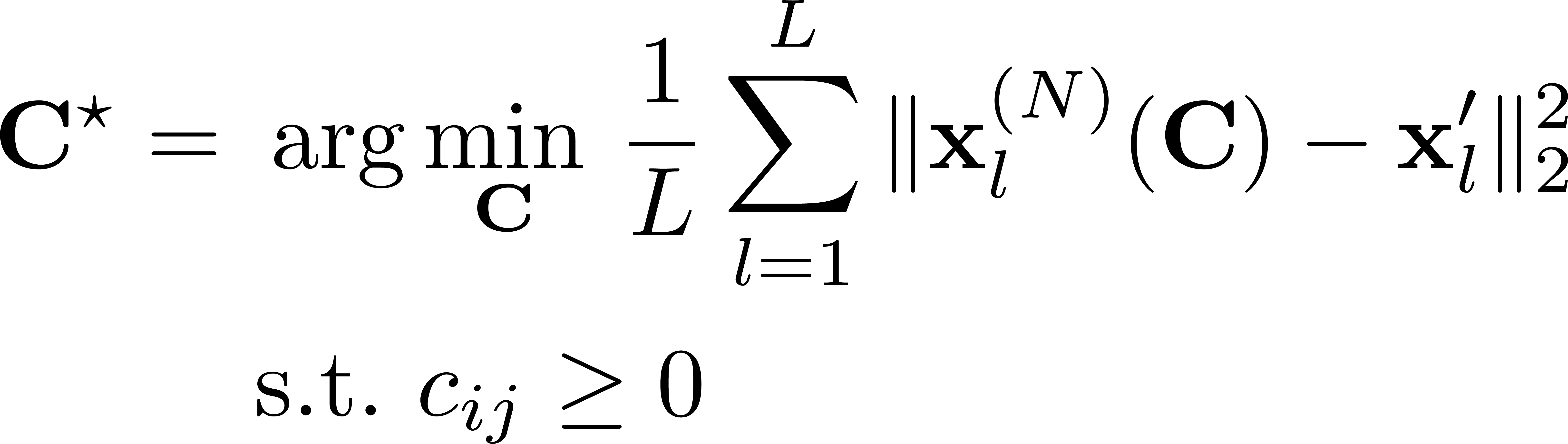
where, our loss function is the $L_2$ distance between the reconstructed phase image, $\mathbf{x}^{(N)}$, and the ground truth, $\mathbf{x}’$, over a small simulated dataset. The LED brightnesses, $C \in \mathbb{R}^{M \times T}$ for $M$ measurements and $T$ LEDs, are constrained to be positive so that our learned designs can be feasibly implemented in hardware. Finally, because the network is only parameterized by a few variables, we can efficiently learn them using a small dataset ($100$ examples)! We minimize the loss function using projected gradient descent.
Experiments
Our experimental context is cell imaging, so we use 100 cell images (100px by 100px) as our dataset (90 training examples / 10 testing examples). We learn the experimental design parameters for acquiring only two measurements. In figure 5, we compare the phase image reconstructions using our learned design [1] and the traditional design against the phase image reconstructed using a validation method. Using only a fraction of the measurements, our learned designs can reconstruct a phase image with a similar quality to that of the validation method, while the traditional design’s phase image is degraded in quality.
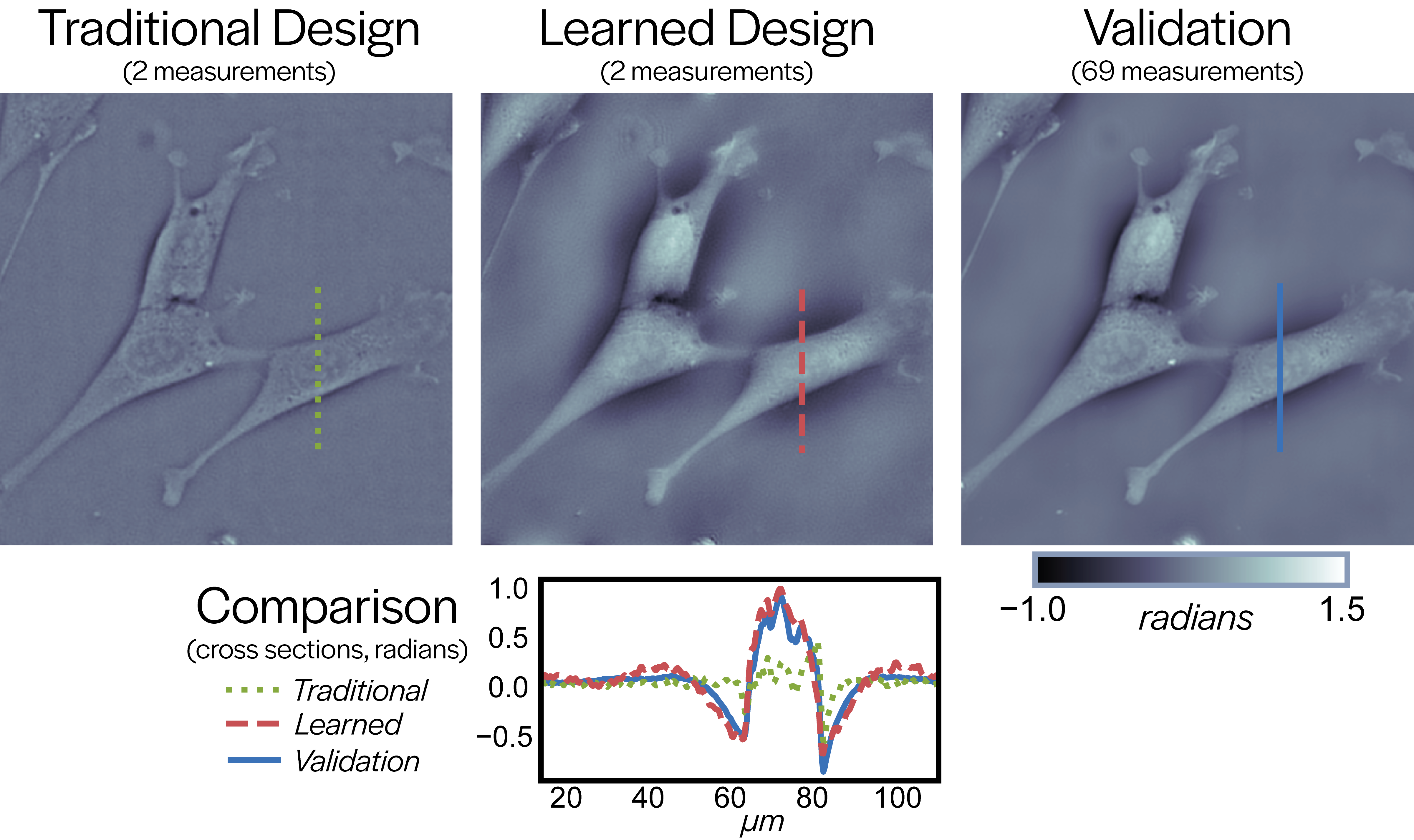
Figure 5: Result Comparison: Quantitative Phase Images of Mouse
Fibroblast Cells reconstructed using (left) traditional design, (middle) our
learned design, and (right) a validation method using many more measurements. Below is
a cross section comparison of the three reconstructions through the nucleus of a
cell.
Conclusion
Optimal experimental design methods are useful when the system is linear; however, their design will not necessarily improve the performance when the system is non-linear. We have shown we can optimize the experimental design for a non-linear computational imaging system using supervised learning and an unrolling physics-based network. Looking forward, we will consider analyzing larger more complex systems with different measurement constraints, as well as, structured ways to learn parts of the image reconstruction.
References
[1] Kellman, M. R., Bostan, E., Repina, N., & Waller, L. (2018). Physics-based Learned Design: Optimized Coded-Illumination for Quantitative Phase Imaging. arXiv preprint arXiv:1808.03571.
[2] Hammernik, K., Klatzer, T., Kobler, E., Recht, M. P., Sodickson, D. K., Pock, T., & Knoll, F. (2018). Learning a variational network for reconstruction of accelerated MRI data. Magnetic resonance in medicine, 79(6), 3055-3071.