Deep imitation learning and deep reinforcement learning have potential to learn robot control policies that map high-dimensional sensor inputs to controls. While these approaches have been very successful at learning short duration tasks, such as grasping (Pinto and Gupta 2016, Levine et al. 2016) and peg insertion (Levine et al. 2016), scaling learning to longer time horizons can require a prohibitive amount of demonstration data—whether acquired from experts or self-supervised. Long-duration sequential tasks suffer from the classic problem of “temporal credit assignment”, namely, the difficulty in assigning credit (or blame) to actions under uncertainty of the time when their consequences are observed (Sutton 1984). However, long-term behaviors are often composed of short-term skills that solve decoupled subtasks. Consider designing a controller for parallel parking where the overall task can be decomposed into three phases: pulling up, reversing, and adjusting. Similarly, assembly tasks can often be decomposed into individual steps based on which parts need to be manipulated. These short-term skills can be parametrized more concisely—as an analogy, consider locally linear approximations to an overall nonlinear function—and this reduced parametrization can be substantially easier to learn.

This post summarizes results from three recent papers that propose algorithms that learn to decompose a longer task into shorter subtasks. We report experiments in the context of autonomous surgical subtasks and we believe the results apply to a variety of applications from manufacturing to home robotics. We present three algorithms: Transition State Clustering (TSC), Sequential Windowed Inverse Reinforcement Learning (SWIRL), and Deep Discovery of Continuous Options (DDCO). TSC considers robustly learning important switching events (significant changes in motion) that occur across all demonstrations. SWIRL proposes an algorithm that approximates a value function by a sequence of shorter term quadratic rewards. DDCO is a general framework for imitation learning with a hierarchical representation of the action space. In retrospect, all three algorithms are special cases of the same general framework, where the demonstrator’s behavior is generatively modeled as a sequential composition of unknown closed-loop policies that switch when reaching parameterized “transition states”.

Application to Surgical Robotics

Robots such as Intuitive Surgical’s da Vinci have facilitated millions of surgical procedures worldwide using local teleoperation. Automation of surgical sub-tasks has the potential to reduce surgeon tedium and fatigue, operating time, and enable supervised tele-surgery over higher-latency networks. Designing surgical robot controllers is particularly difficult due to a limited field of view and imprecise actuation.

As a concrete task, pattern cutting is one of the Fundamentals of Laparoscopic Surgery, a training suite required of surgical residents. In this standard surgical training task, the surgeon must cut and remove a pattern printed on a sheet of gauze, and is scored on time and accuracy:

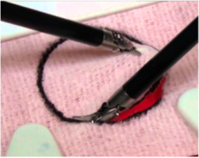
Pattern cutting task from the Fundamentals of Laparoscopic Surgery.

In (Murali 2015), we manually coded this task using hand-crafted Deterministic Finite Automaton on the da Vinci surgical robot. The DFA integrated 10 different manipulation primitives and two computer vision based checks:

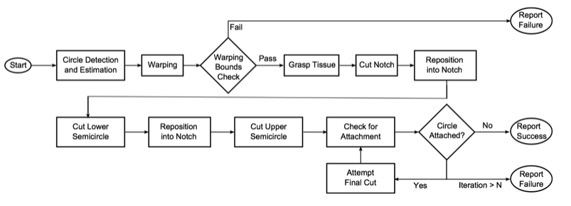
Deterministic finite automaton from Murali et al. 2016 to automate pattern cutting.

Designing this DFA required painstaking trial-and-error, and perceptual checks required constant tuning to account for lighting and registration changes. This motivated us to consider the extent to which we could learn such structure from demonstration data. This blog post describes our efforts over the last three years at learning hierarchical representations from demonstrations. This research has helped us automate several surgical robotic tasks with minimal expert design of the DFA, as shown in the three GIFs at the top of the post.

Learning Transition Conditions

The first paper, Transition State Clustering (Krishnan et al. 2015), explores the problem of learning transition conditions from demonstrations, i.e., conditions that trigger a switch or a transition between manipulation behaviors in a task. In many important tasks, while the actual motions may vary and be noisy, each demonstration contains roughly the same sequence of primitive motions. This consistent, repeated structure can be exploited to infer global transition criteria by identifying state-space conditions correlated with significant changes in motion. By assuming a known sequential order of primitives, the problem reduces to segmenting each trajectory and corresponding those segments across trajectories. This involves finding a common set of segment-to-segment transition events.

We formalized this intuition in an algorithm called Transition State Clustering (TSC). Let \(D=\{d_i\}\) be a set of demonstrations of a robotic task. Each demonstration of a task $d$ is a discrete-time sequence of $T$ state vectors in a feature-space $\mathcal{X}$. The feature space is a concatenation of kinematic features $X$ (e.g., robot position) and sensory features $V$. These were low-dimensional visual features from the environment calculated by hard-coded image processing and manual annotation.

A segmentation of a task is defined as a function $\mathcal{S}$ that maps each trajectory to a non-decreasing sequence of integers in ${1,2,…,k}$. This function tells us more than just the endpoints of segments, since it also labels each segment according to its sub-task. By contrast, a transition indicator function $\mathcal{T}$ is maps each demonstration $d$ to a sequence of indicators in ${0,1}$:

such that \(\mathcal{T}(d)_t\) indicates whether the demonstration switched from one sub-task to another after time $t$. For a demonstration $d_i$, let $o_{i,t}$ denote the kinematic state, visual state, and time $(x,v,t)$ at time $t$. Transition States are the set of state-time tuples where the indicator is 1:

In TSC, we model the probability distribution that generates $\Gamma$ as a Gaussian Mixture Model and identify the mixture components. These components identify regions of the state space correlated with candidate transitions. We can take any motion-based model for detecting changes in behavior and generate candidates. Then, we probabilistically ground these candidate transitions in state-space and perceptual conditions that are consistent across demonstrations. Intuitively, this algorithm consists of two steps: first segmentation, and then clustering the segment end-points.

There are a number of important implementation details to make this model work in practice on real noisy data. Since the kinematic and visual features often have very different scales and topological properties, we often have to model them separately during the clustering step. We hierarchically apply a GMM model by first performing a hard clustering on the kinematic features, and then within each cluster fitting the probabilistic model over the perceptual features. This allows us to prune out clusters that are not representative (i.e., do not have transitions from all demonstrations). Furthermore, Hyper-parameter selection is a known problem in mixture models. Recent results in Bayesian statistics can mitigate some of these problems by defining a soft prior of the number of mixtures. The Dirichlet Process (DP) defines a distribution over the parameters of discrete distributions, in our case, the probabilities of a categorical distribution, as well as the size of its support $m$ (Kulis 2011). The hyper-parameters of the DP can be inferred with variational Expectation Maximization.

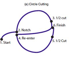
In the pattern cutting task, TSC found the following transition conditions:

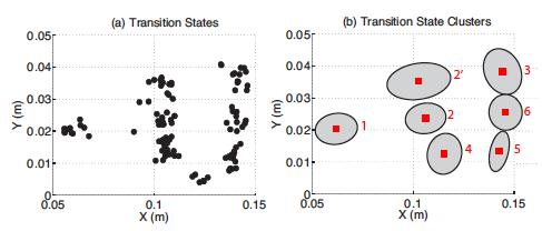
Surgical pattern cutting task. Left: manually identified transitions. Right: automatically discovered transition states (a) and transition state clusters (b).

We marked 6 manually identified primitive motions from (Murali et al. 2015): (1) start, (2) notch, (3) finish 1st cut, (4) cross-over, (5) finish 2nd cut, and (6) connect the two cuts. TSC automatically identifies 7 segments, which correspond well to our prior work. It is worth noting that there is one extra cluster (marked 2’), that does not correspond to a transition in the manual segmentation.

At 2’, the operator finishes a notch and begins to cut. While at a logical level, notching and cutting are both penetration actions, they correspond to two different motion regimes due to the positioning of the end-effector. TSC separates them into different clusters even though the human annotators overlooked this important transition.

Connection to Inverse Reinforcement Learning

We next explored how the transitions learned by TSC can be used to shape rewards in long horizon tasks. Sequential Windowed Inverse Reinforcement Learning (Krishnan et al. 2016), models a task as a sequence of quadratic reward functions

and transition regions

such that $R_1$ is the reward function until $\rho_1$ is reached, after which $R_2$ becomes the reward and so on.

We assume that we have access to a supervisor that provides demonstrations which are optimal w.r.t an unknown reward function $\mathbf{R}^*$ (not necessarily quadratic), and which reach each $\rho \in G$ (also unknown) in the same order. SWIRL is an algorithm to recover \(\mathbf{R}_{seq}\) and $G$ from the demonstration trajectories. SWIRL applies to tasks with a discrete or continuous state-space and a discrete action-space. The state space can represent spatial, kinematic, or sensory states (e.g., visual features), as long as the trajectories are smooth and not very high-dimensional. Finally, $\mathbf{R}_{seq}$ and $G$ can be used in an RL algorithm to find an optimal policy for a task.

TSC can be interpreted as inferring the subtask transition regions $G$. Once the transitions are found, SWIRL applies Maximum Entropy Inverse Reinforcement Learning to find a local quadratic reward function that guides the robot to the transition condition. Segmentation further simplifies the estimation of dynamics models, which are required for inference in MaxEnt-IRL, since many complex systems can be locally approximated linearly in a short time horizon. The goal of MaxEnt-IRL is to find a reward function such that an optimal policy w.r.t that reward function is close to the expert demonstration. The agent is modeled as nosily optimal, where it takes actions from a policy $\pi$:

$A_\theta$ is the advantage function (gap between the values of action $a$ and of the optimal action in state $s$) for the reward parametrized by $\theta$. The objective is to maximize the log-likelihood that the demonstration trajectories were generated by $\theta$. In MaxEnt-IRL, this objective can be estimated reliably in two cases, discrete and linear-Gaussian systems, since it requires an efficient forward search of the policy given a particular reward parametrized by $\theta$. Thus, we assume that our demonstrations can be modeled either discretely or with linear dynamics.

Learning a policy from $\mathbf{R}_{seq}$ and $G$ is nontrivial because solving $k$ independent problems neglects any shared structure in the value function during the policy learning phase (e.g., a common failure state). Jointly learning over all segments introduces a dependence on history, namely, any policy must complete step $i$ before step $i+1$. Learning a memory-dependent policy could lead to an exponential overhead of additional states. SWIRL exploits the fact that TSC is in a sense a Markov process, and shows that the problem can be posed as a proper MDP in a lifted state-space that includes an indicator variable of the highest-index ${1,…,k}$ transition region that has been reached so far.

SWIRL applies a variant of Q-Learning to optimize the policy over the sequential rewards. The basic change to the algorithm is to augment the state-space with an indicator vector that indicates the transition regions that have been reached. Each of the rollouts now records a tuple

that additionally stores this information. The Q function is now defined over states, actions, and segment index–which also selects the appropriate local reward function:

We also need to define an exploration policy, i.e., a stochastic policy with which we will collect rollouts. To initialize the Q-Learning, we apply Behavioral Cloning locally for each of the segments to get a policy $\pi_i$. We apply an $\epsilon$-greedy version of these policies to collect rollouts.

We evaluated SWIRL on a deformable sheet tensioning task. A sheet of surgical gauze is fixtured at the two far corners using a pair of clips. The unclipped part of the gauze is allowed to rest on soft silicone padding. The robot’s task is to reach for the unclipped part, grasp it, lift the gauze, and tension the sheet to be as planar as possible. An open-loop policy, one that does not react to unexpected changes, typically fails on this task because it requires some feedback of whether gauze is properly grasped, how the gauze has deformed after grasping, and visual feedback of whether the gauze is planar. The task is sequential, as some grasps pick up more or less of the material and the flattening procedure has to be accordingly modified.

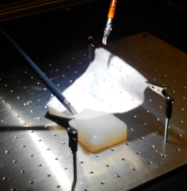
Deformable sheet tensioning setup.

We provided 15 demonstrations through a keyboard-based tele-operation interface. The average length of the demonstrations was 48.4 actions (although we sampled observations at a higher frequency, about 10 observations for every action). From these 15 demonstrations, SWIRL identifies four segments. One of the segments corresponds to moving to the correct grasping position, one corresponds to making the grasp, one lifting the gauze up again, and one corresponds to straightening the gauze. One of the interesting aspects of this task is that the segmentation requires multiple features, and segmenting any single signal may miss an important feature.

Then, we tried to learn a policy from the rewards constructed by SWIRL. We define a Q-Network with a single-layer Multi-Layer Perceptron with 32 hidden units and sigmoid activation. For each of the segments, we apply Behavioral Cloning locally with the same architecture as the Q-network (with an additional softmax over the output layer) to get an initial policy. We roll out 100 trials with an $\epsilon=0.1$ greedy version of these segmented policies. The results are depicted below:

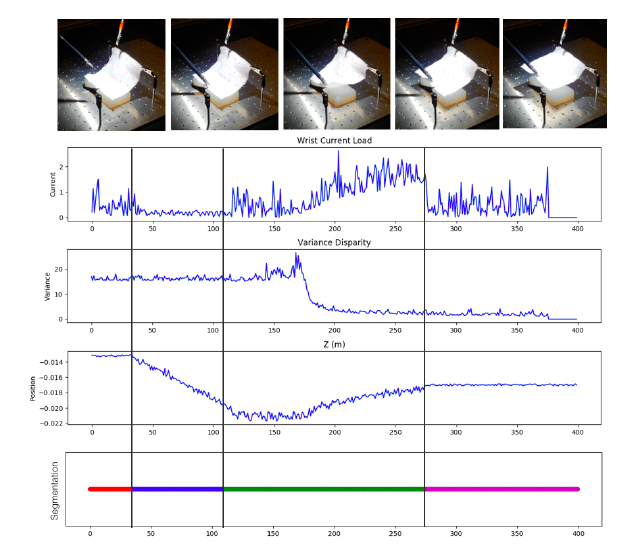
A representative demonstration of the deformable sheet tensioning task with relevant features plotted over time. SWIRL identifies 4 segments which correspond to reaching, grasping, lifting, and tensioning.

SWIRL achieves more than a 4 times higher reward than ab initio RL, 3 time higher than pure behavioral cloning, and a 56% higher reward than naively applying behavioral cloning with TSC segments.

Hierarchical Representations

We are now exploring a generalization of TSC and SWIRL with a new algorithm: Deep Discovery of Continuous Options (DDCO Krishnan et al. 2017, to be presented at the 1st Conference on Robot Learning in November).

An option represents a low-level policy that can be invoked by a high-level policy to perform a certain sub-task. Formally, an option $h$ in an options set $\mathcal H$ is specified by a control policy $\pi_h(a_t | s_t)$ and a stochastic termination condition $\psi_h(s_t)\in[0,1]$. The high-level policy $\eta(h_t | s_t)$ defines the distribution over options given the state. Once an option $h$ is invoked, physical controls are selected by the option’s policy $\pi_h$ until it terminates. After each physical control is applied and the next state $s’$ is reached, the option $h$ terminates with probability $\psi_h(s’)$, and if it does then the high-level policy selects a new option $h’$ with distribution $\eta(h’ | s’)$. Thus the interaction of the hierarchical control policy $\langle\eta,(\pi_h,\psi_h)_{h\in\mathcal H}\rangle$ with the system induces a stochastic process over the states $s_t$, the options $h_t$, the controls $a_t$, and the binary termination indicators $b_t$.

DDCO is a policy-gradient algorithm that discovers parametrized options by fitting their parameters to maximize the likelihood of a set of demonstration trajectories. We denote by $\theta$ the vector of all trainable parameters used for $\eta$ and for $\pi_h$ and $\psi_h$ of each option $h\in\mathcal H$. For example, $\theta$ can be the weights and biases of a feed-forward network that computes these probabilities. We wish to find the $\theta\in\Theta$ that maximizes the log-likelihood of generating each demonstration trajectory $\xi=(s_0,a_0,s_1,\ldots,s_T)$. The challenge is that this log-likelihood depends on the latent variables in the stochastic process, the options and the termination indicators $\zeta = (b_0,h_0,b_1,h_1,\ldots,h_{T-1})$. DDCO optimizes this objective with an Expectation-Gradient algorithm:

where $\mathbb{P}_\theta(\zeta,\xi)$ is the joint probability of the latent and observable variables, given by

where in the latent transition \(\mathbb{P}_\theta(b_t, h_t | h_{t-1}, s_t)\) we have with probability $\psi_{h_{t-1}}(s_t)$ that $b_t=1$ and $h_t$ is drawn from $\eta(\cdot|s_t)$, and otherwise that $b_t=0$ and $h_t$ is unchanged, i.e.

The log-likelihood gradient can be computed in two steps, an E-step where the marginal posteriors

are computed using a forward-backward algorithm similar to Baum-Welch, and a G-step:

The gradient computed above can then be used in any stochastic gradient descent algorithm. In our experiments we use Adam and Momentum.

We evaluated DDCO in an Imitation Learning setting with surgical robotic tasks. In one task, the robot is given a foam bin with a pile of 5–8 needles of three different types, each 1–3mm in diameter. The robot must extract needles of a specified type and place them in an “accept” cup, while placing all other needles in a “reject” cup. The task is successful if the entire foam bin is cleared into the correct cups. To define the state space for this task, we first generate binary images from overhead stereo images, and apply a color-based segmentation to identify the needles (the “image” input). Then, we use a classifier trained in advance on 40 hand-labeled images to identify and provide a candidate grasp point, specified by position and direction in image space (the “grasp” input). Additionally, the 6 DoF robot gripper pose and the open-closed state of the gripper are observed (the “kin” input). The state space of the robot is (“image”, “grasp”, “kin”), and the control space is the 6 joint angles and the gripper angle.

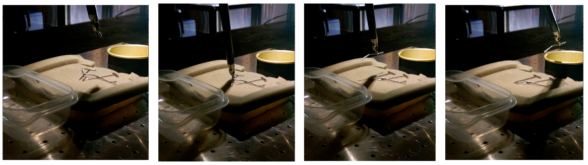
Needle pick and place task on the surgical robot.

In 10 trials, 7/10 were successful. The main failure mode was unsuccessful grasping due to picking either no needles or multiple needles. As the piles were cleared and became sparser, the robot’s grasping policy became somewhat brittle. The grasp success rate was 66% on 99 attempted grasps. In contrast, we rarely observed failures at the other aspects of the task, reaching 97% successful recovery on 34 failed grasps.

The learned options are interpretable on intuitive task boundaries. For each of the 4 options, we plot how heavily the different inputs are weighted (image, grasp, or kin) in computing the option’s action. Nonzero values of the ReLU units are marked in white and indicate input relevance:

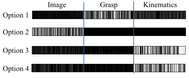
We plot the average activations of the feature layer for of each option, indicating which inputs (image, gripper angle, or kinematics ) are relevant to the policy and termination.

We see that the options are clearly specialized. The first option has a strong dependence only on the grasp candidate, the second option attends almost exclusively to the image, while the last two options rely mostly on the kinematics and grasp features.

Conclusion

To summarize, learning sequential task structure from demonstrations has many applications in robotics such as automating surgical sub-tasks and can be facilitated by segmenting to learning task structure. We see several avenues for future work: (1) representations that better model rotational geometry and configuration spaces, (2) hybrid schemes that consider both parametrized primitives and those derived from analytic formulae, and (3) consideration of state-space segmentation as well as temporal segmentation.

References

(For links to papers, see the homepages of Sanjay Krishnan or Ken Goldberg.)

Sanjay Krishnan*, Roy Fox*, Ion Stoica, Ken Goldberg. DDCO: Discovery of Deep Continuous Options for Robot Learning from Demonstrations. Conference on Robot Learning (CoRL). 2017.

Sanjay Krishnan, Animesh Garg, Richard Liaw, Brijen Thananjeyan, Lauren Miller, Florian T. Pokorny, Ken Goldberg. SWIRL: A Sequential Windowed Inverse Reinforcement Learning Algorithm for Robot Tasks With Delayed Rewards. Workshop on Algorithmic Foundations of Robotics (WAFR) 2016.

Sanjay Krishnan*, Animesh Garg*, Sachin Patil, Colin Lea, Gregory Hager, Pieter Abbeel, Ken Goldberg. Transition State Clustering: Unsupervised Surgical Task Segmentation For Robot Learning. International Symposium on Robotics Research (ISRR). 2015.

Adithyavairavan Murali*, Siddarth Sen*, Ben Kehoe, Animesh Garg, Seth McFarland, Sachin Patil, W. Douglas Boyd, Susan Lim, Pieter Abbeel, Ken Goldberg. Learning by Observation for Surgical Subtasks: Multilateral Cutting of 3D Viscoelastic and 2D Orthotropic Tissue Phantoms. International Conference on Robotics and Automation (ICRA). May 2015.

External References

Richard Sutton. Temporal credit assignment in reinforcement learning. 1984.

Richard Sutton, Doina Precup, and Satinder Singh. Between MDPs and semi-MDPs: A framework for temporal abstraction in reinforcement learning. Artificial intelligence. 1999.

Lerrel Pinto, and Abhinav Gupta. Supersizing self-supervision: Learning to grasp from 50k tries and 700 robot hours. International Conference on Robotics and Automation (ICRA). 2016.

Sergey Levine, Peter Pastor, Alex Krizhevsky, Julian Ibarz, Deirdre Quillen. Learning Hand-Eye Coordination for Robotic Grasping with Deep Learning and Large-Scale Data Collection (International Journal of Robotics Research). 2017.

Sergey Levine*, Chelsea Finn*, Trevor Darrell, and Pieter Abbeel. End-to-end training of deep visuomotor policies. Journal of Machine Learning Research (JMLR). 2016.