Over the last few years we have experienced an enormous data deluge, which has played a key role in the surge of interest in AI. A partial list of some large datasets:

• ImageNet, with over 14 million images for classification and object detection.
• Movielens, with 20 million user ratings of movies for collaborative filtering.
• Udacity’s car dataset (at least 223GB) for training self-driving cars.
• Yahoo’s 13.5 TB dataset of user-news interaction for studying human behavior.

Stochastic Gradient Descent (SGD) has been the engine fueling the development of large-scale models for these datasets. SGD is remarkably well-suited to large datasets: it estimates the gradient of the loss function on a full dataset using only a fixed-sized minibatch, and updates a model many times with each pass over the dataset.

But SGD has limitations. When we construct a model, we use a loss function $L_\theta(x)$ with dataset $x$ and model parameters $\theta$ and attempt to minimize the loss by gradient descent on $\theta$. This shortcut approach makes optimization easy, but is vulnerable to a variety of problems including over-fitting, excessively sensitive coefficient values, and possibly slow convergence. A more robust approach is to treat the inference problem for $\theta$ as a full-blown posterior inference, deriving a joint distribution $p(x,\theta)$ from the loss function, and computing the posterior $p(\theta|x)$. This is the Bayesian modeling approach, and specifically the Bayesian Neural Network approach when applied to deep models. This recent tutorial by Zoubin Ghahramani discusses some of the advantages of this approach.

The model posterior $p(\theta|x)$ for most problems is intractable (no closed form). There are two methods in Machine Learning to work around intractable posteriors: Variational Bayesian methods and Markov Chain Monte Carlo (MCMC). In variational methods, the posterior is approximated with a simpler distribution (e.g. a normal distribution) and its distance to the true posterior is minimized. In MCMC methods, the posterior is approximated as a sequence of correlated samples (points or particle densities). Variational Bayes methods have been widely used but often introduce significant error — see this recent comparison with Gibbs Sampling, also Figure 3 from the Variational Autoencoder (VAE) paper. Variational methods are also more computationally expensive than direct parameter SGD (it’s a small constant factor, but a small constant times 1-10 days can be quite important).

MCMC methods have no such bias. You can think of MCMC particles as rather like quantum-mechanical particles: you only observe individual instances, but they follow an arbitrarily-complex joint distribution. By taking multiple samples you can infer useful statistics, apply regularizing terms, etc. But MCMC methods have one over-riding problem with respect to large datasets: other than the important class of conjugate models which admit Gibbs sampling, there has been no efficient way to do the Metropolis-Hastings tests required by general MCMC methods on minibatches of data (we will define/review MH tests in a moment). In response, researchers had to design models to make inference tractable, e.g. Restricted Boltzmann Machines (RBMs) use a layered, undirected design to make Gibbs sampling possible. In a recent breakthrough, VAEs use variational methods to support more general posterior distributions in probabilistic auto-encoders. But with VAEs, like other variational models, one has to live with the fact that the model is a best-fit approximation, with (usually) no quantification of how close the approximation is. Although they typically offer better accuracy, MCMC methods have been sidelined recently in auto-encoder applications, lacking an efficient scalable MH test.

A bridge between SGD and Bayesian modeling has been forged recently by papers on Stochastic Gradient Langevin Dynamics (SGLD) and Stochastic Gradient Hamiltonian Monte Carlo (SGHMC). These methods involve minor variations to typical SGD updates which generate samples from a probability distribution which is approximately the Bayesian model posterior $p(\theta|x)$. These approaches turn SGD into an MCMC method, and as such require Metropolis-Hastings (MH) tests for accurate results, the topic of this blog post.

Because of these developments, interest has warmed recently in scalable MCMC and in particular in doing the MH tests required by general MCMC models on large datasets. Normally an MH test requires a scan of the full dataset and is applied each time one wants a data sample. Clearly for large datasets, it’s intractable to do this. Two papers from ICML 2014, Korattikara et al. and Bardenet et al., attempt to reduce the cost of MH tests. They both use concentration bounds, and both achieve constant-factor improvements relative to a full dataset scan. Other recent work improves performance but makes even stronger assumptions about the model which limits applicability, especially for deep networks. None of these approaches come close to matching the performance of SGD, i.e. generating a posterior sample from small constant-size batches of data.

In this post we describe a new approach to MH testing which moves the cost of MH testing from $O(N)$ to $O(1)$ relative to dataset size. It avoids the need for global statistics and does not use tail bounds (which lead to long-tailed distributions for the amount of data required for a test). Instead we use a novel correction distribution to directly “morph” the distribution of a noisy minibatch estimator into a smooth MH test distribution. Our method is a true “black-box” method which provides estimates on the accuracy of each MH test using only data from a small expected size minibatch. It can even be applied to unbounded data streams. It can be “piggy-backed” on existing SGD implementations to provide full posterior samples (via SGLD or SGHMC) for almost the same cost as SGD samples. Thus full Bayesian neural network modeling is now possible for about the same cost as SGD optimization. Our approach is also a potential substitute for variational methods and VAEs, providing unbiased posterior samples at lower cost.

To explain the approach, we review the role of MH tests in MCMC models.

Markov Chain Monte Carlo Review

Markov Chains

MCMC methods are designed to sample from a target distribution which is difficult to compute. To generate samples, they utilize Markov Chains, which consist of nodes representing states of the system and probability distributions for transitioning from one state to another.

A key concept is the Markovian assumption, which states that the probability of being in a state at time $t+1$ can be inferred entirely based on the current state at time $t$. Mathematically, letting $\theta_t$ represent the current state of the Markov chain at time $t$, we have $p(\theta_{t+1} | \theta_t, \ldots, \theta_0) = p(\theta_{t+1} | \theta_t)$. By using these probability distributions, we can generate a chain of samples $(\theta_i)_{i=1}^T$ for some large $T$.

Since the probability of being in state $\theta_{t+1}$ directly depends on $\theta_t$, the samples are correlated. Rather surprisingly, it can be shown that, under mild assumptions, in the limit of many samples the distribution of the chain’s samples approximates the target distribution.

A full review of MCMC methods is beyond the scope of this post, but a good reference is the Handbook of Markov Chain Monte Carlo (2011). Standard machine learning textbooks such as Koller & Friedman (2009) and Murphy (2012) also cover MCMC methods.

Metropolis-Hastings

One of the most general and powerful MCMC methods is Metropolis-Hastings. This uses a test to filter samples. To define it properly, let $p(\theta)$ be the target distribution we want to approximate. In general, it’s intractable to sample directly from it. Metropolis-Hastings uses a simpler proposal distribution $q(\theta’ | \theta)$ to generate samples. Here, $\theta$ represents our current sample in the chain, and $\theta’$ represents the proposed sample. For simple cases, it’s common to use a Gaussian proposal centered at $\theta$.

If we were to just use a Gaussian to generate samples in our chain, there’s no way we could approximate our target $p$, since the samples would form a random walk. The MH test cleverly resolves this by filtering samples with the following test. Draw a uniform random variable $u \in [0,1]$ and determine whether the following is true:

If true, we accept $\theta’$. Otherwise, we reject and reuse the old sample $\theta$. Notice that

• It doesn’t require knowledge of a normalizing constant (independent of $\theta$ and $\theta’$), because that cancels out in the $p(\theta’)/p(\theta)$ ratio. This is great, because normalizing constants are arguably the biggest reason why distributions become intractable.
• The higher the value of $p(\theta’)$, the more likely we are to accept.

To get more intuition on how the test works, we’ve created the following figure from this Jupyter Notebook, showing the progression of samples to approximate a target posterior. This example is derived from Welling & Teh (2011).

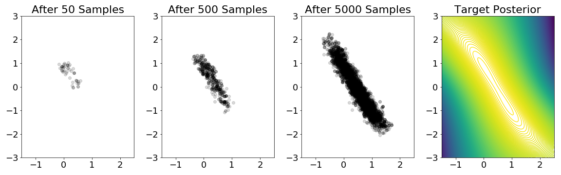
A quick example of the MH test in action on a mixture of Gaussians example. The parameter is $\theta \in \mathbb{R}^2$ with the x and y axes representing $\theta_1$ and $\theta_2$, respectively. The target posterior has contours shown in the fourth plot; the probability mass is concentrated in the diagonal between points $(0,1)$ and $(1,-1)$. (This posterior depends on sampled Gaussians.) The plots show the progression of the MH test after 50, 500, and 5000 samples in our MCMC chain. After 5000 samples, it's clear that our samples are concentrated in the regions with higher posterior probability.

Reducing Metropolis-Hastings Data Usage

What happens when we consider the Bayesian posterior inference case with large datasets? (Perhaps we’re interested in the same example in the figure above, except that the posterior is based on more data points.) Then our goal is to sample to approximate the distribution $p(\theta | x_1, \ldots, x_N)$ for large $N$. By Bayes’ rule, this is $\frac{p_0(\theta)p(x_1, \ldots, x_N | \theta) }{p(x_1,\ldots,x_N)}$ where $p_0$ is the prior. We additionally assume that the $x_i$ are conditionally independent given $\theta$. The MH test therefore becomes:

Or, after taking logarithms and rearranging (while ignoring the minimum operator, which technically isn’t needed here), we get

The problem now is apparent: it’s expensive to compute all the $p(x_i | \theta’)$ terms, and this has to be done every time we sample since it depends on $\theta’$.

The naive way to deal with this is to apply the same test, but with a minibatch of $b$ elements:

Unfortunately, this won’t sample from the correct target distribution; see Section 6.1 in Bardenet et al. (2017) for details.

A better strategy is to start with the same batch of $b$ points, but then gauge the confidence of the batch test relative to using the full data. If, after seeing $b$ points, we already know that our proposed sample $\theta’$ is significantly worse than our current sample $\theta$, then we should reject right away. If $\theta’$ is significantly better, we should accept. If it’s ambiguous, then we increase the size of our test batch, perhaps to $2b$ elements, and then measure the test’s confidence. Lather, rinse, repeat. As mentioned earlier, Korattikara et al. (2014) and Bardenet et al. (2014) developed algorithms following this framework.

A weakness of the above approach is that it’s doing repeated testing and one must reduce the allowable test error each time one increments the test batch size. Unfortunately, there is also a significant probability that the approaches above will grow the test batch all the way to the full dataset, and they offer at most constant factor speedups over testing the full dataset.

Minibatch Metropolis-Hastings: Our Contribution

Change the Acceptance Function

To set up our test, we first define the log transition probability ratio $\Delta$:

This log ratio factors into a sum of per-sample terms, so when we approximate its value by computing on a minibatch we get an unbiased estimator of its full-data value plus some noise (which is asymptotically normal by the Central Limit Theorem).

The first step for applying our MH test is to use a different acceptance function. Expressed in terms of $\Delta$, the classical MH accepts a transition with probability given by the blue curve.

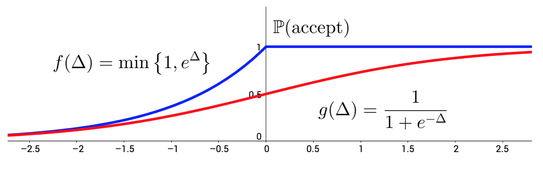
Functions $f$ and $g$ can serve as acceptance tests for Metropolis-Hastings. Given current sample $\theta$ and proposed sample $\theta'$, the vertical axis represents the probability of accepting $\theta'$.

Instead of using the classical test, we’ll use the sigmoid function. It might not be apparent why this is allowed, but there’s some elegant theory that explains why using this alternative function as the acceptance test for MH still results in the correct semantics of MCMC. That is, under the same mild assumptions, the distribution of samples $(\theta_i)_{i=1}^T$ approaches the target distribution.

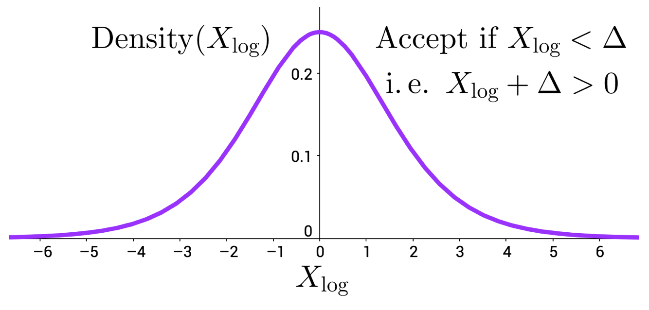
The density of the standard logistic random variable, denoted $X_{\rm log}$ along with the equivalent MH test expression ($X_{\rm log}+\Delta > 0$) with the sigmoid acceptance function.

Our acceptance test is now the sigmoid function. Note that the sigmoid function is the cumulative distribution function of a (standard) Logistic random variable; the figure above plots the density. One can show that the MH test under the sigmoid acceptance function reduces to determining whether $X_{\rm \log} + \Delta > 0$ for a sampled $X_{\rm log}$ value.

New MH Test

This is nice, but we don’t want to compute $\Delta$ because it depends on all $p(x_i | \theta’)$ terms. When we estimate $\Delta$ using a minibatch, we introduce an additive error which is approximately normal, $X_{\rm normal}$. The key observation in our work is that the distribution of the minibatch estimate of $\Delta$ (approximately Gaussian) is already very close to the desired test distribution $X_{\rm log}$, as shown below.

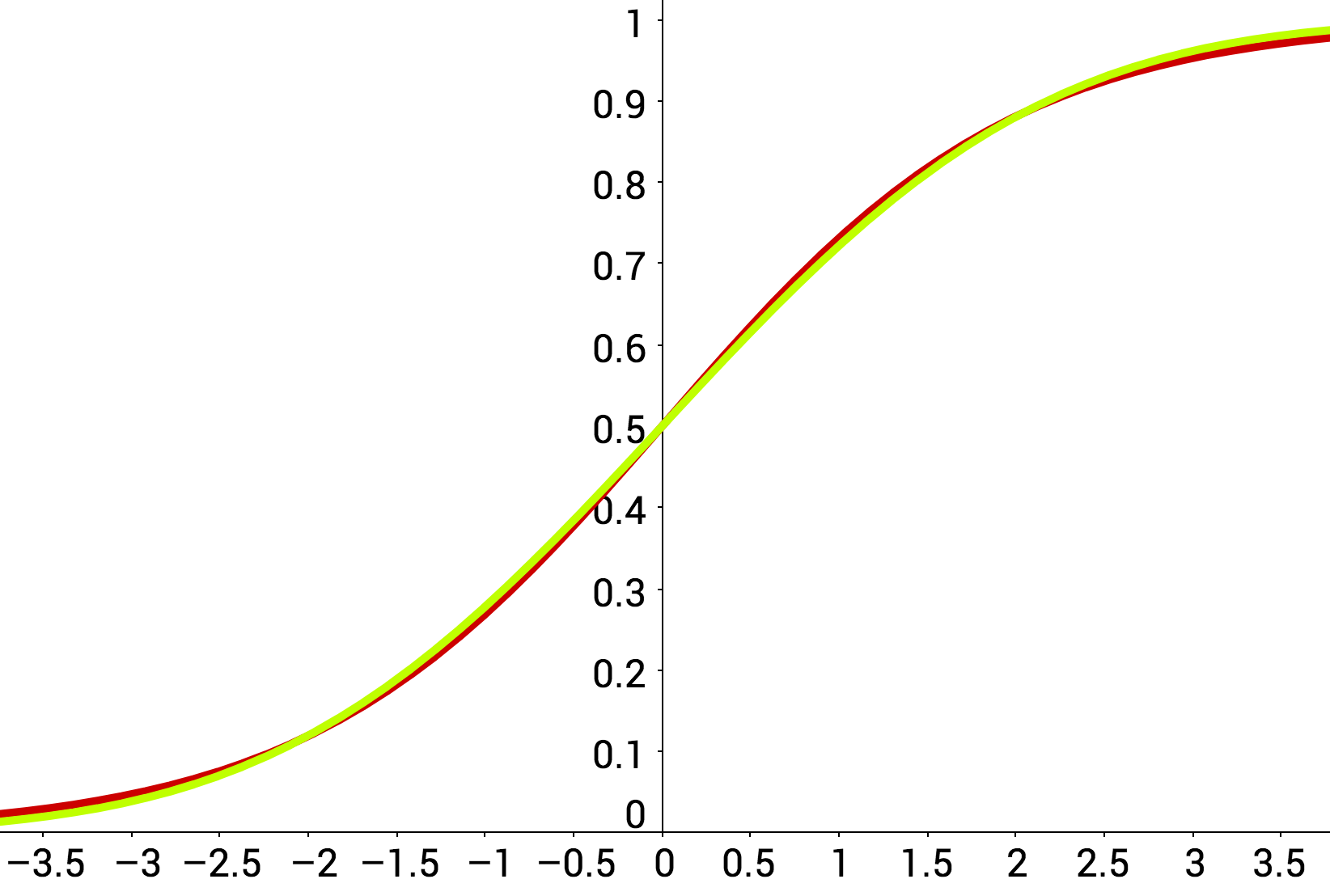
A plot of the logistic CDF in red (as we had earlier) along with a normal CDF curve, colored in lime, which corresponds to a standard deviation of 1.7.

Rather than resorting to tail bounds as in prior work, we directly bridge these two distributions using an additive correction variable $X_{\rm correction}$:

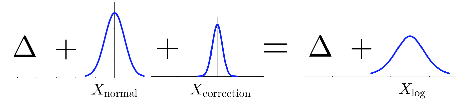
A diagram of our minibatch MH test. On the right we have the full data test that we want, but we can't use it since $\Delta$ is intractable. Instead, we have $\Delta + X_{\rm normal}$ (from the left side) and must add a correction $X_{\rm correction}$.

We want to make the LHS and RHS distributions equal, so we add in a correction $X_{\rm correction}$ which is a symmetric random variable centered at zero. Adding independent random variables gives a random variable whose distribution is the convolution of the summands’ distributions. So finding the correction distribution involves “deconvolution” of a logistic and normal distribution. It’s not always possible to do this, and several conditions must be met (e.g. the tails of the normal distribution must be weaker than the logistic) but luckily for us they are. In our paper to appear at UAI 2017 we show that the correction distribution can be approximated to essentially single-precision floating-point precision by tabulation.

In our paper, we also prove theoretical results bounding the error of our test, and present experimental results showing that our method results in accurate posterior estimation for a Gaussian Mixture Model, and that it is also highly sample-efficient in Logistic Regression for classification of MNIST digits.

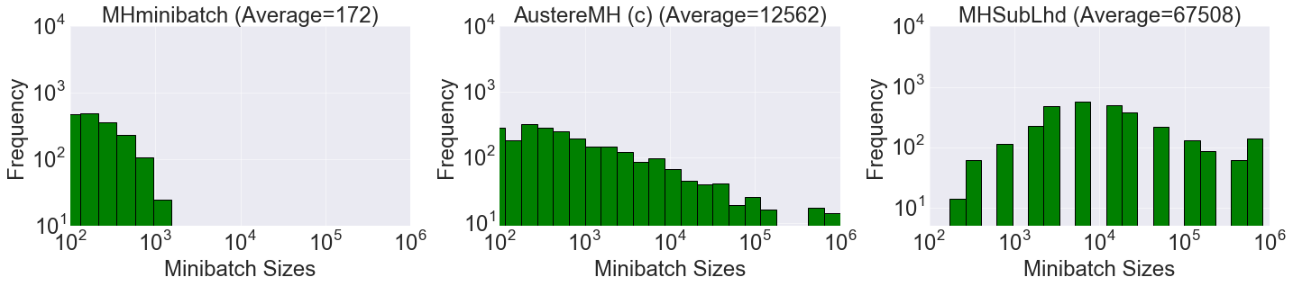
Histograms showing the batch sizes used for Metropolis-Hastings for the three algorithms benchmarked in our paper. The posterior is similar to the earlier example from the Jupyter Notebook, except generated with one million data points. Left is our result, the other two are from Korattikara et al. (2014), and Bardenet et al. (2014), respectively. Our algorithm uses an average of just 172 data points each iteration. Note the log-log scale of the histograms.

We hope our test is useful to other researchers who are looking to use MCMC methods in large datasets. We’ve also implemented an open-source version of the test as part of the BIDMach machine learning library developed at UC Berkeley.

We thank co-authors Xinlei Pan and Haoyu Chen for their help on this project.

• An Efficient Minibatch Acceptance Test for Metropolis-Hastings.
  Daniel Seita, Xinlei Pan, Haoyu Chen, John Canny.
  Uncertainty in Artificial Intelligence, 2017.